?graphics1 Why Base R Graphics in 2026?
1.1 Introduction
Base graphics have a reputation problem. The usual first question about them is some version of isn’t this the old way?, and the usual answer is a shrug. This chapter argues the opposite: in 2026, base graphics are the correct first tool for a specific and fairly large set of jobs, and this book is that tool’s documentation.
In this chapter, we will
- establish what base graphics actually is, and what ships with R
- measure how fast they draw, and how that measurement is usually faked
- measure what a plotting session costs to start
- count the dependencies that
ggplot2adds and base graphics does not - walk a decision tree for choosing between the two
We will do this with numbers rather than adjectives. Every figure in this chapter is produced by a script in scripts/, stored as a CSV in data/, and committed. Nothing here runs when the book is built, which is deliberate: a book that argues for zero dependencies cannot quietly require two of them to prove the point. If a number in this chapter is ever wrong, you can re-run the script that produced it and find out which of us was wrong.
1.2 What “base graphics” means
Base graphics is the set of plotting functions that ship inside R itself, in the graphics package. There is nothing to install.
The package has been part of R since before R 1.0 and its core has barely changed, which is either its greatest strength or its most damning indictment depending on who is talking. The reason it survives is that it does one thing very well: it takes coordinates and draws them. Everything else in this book is an elaboration on that idea.
The key practical fact is this one:
plot(mtcars$disp, mtcars$mpg)
No library() call. graphics is one of the packages R attaches at startup, alongside stats, grDevices, utils and methods. It is not merely available, it is already loaded, which is a stronger guarantee than “cheap to install”. We will quantify that in a moment.
The three systems you are likely to meet in R are:
- base graphics (
graphics) — in R, always present, coordinates in, marks out ggplot2— a large, opinionated package built on the grammar of graphics, with a large dependency treelattice— a Trellis-style system for multivariate data, part of R’s recommended packages
This book is about the first one. Chapter 2 surveys all three.
1.2.1 Why the naming matters
Base graphics is frequently described as “low-level”. That is accurate and slightly misleading in equal measure. The drawing primitives are low-level: plot(), points(), lines(), text(), polygon(), arrows() and rect() put marks at coordinates you choose. But the high-level functions you actually call most often — barplot(), boxplot(), hist(), pairs(), plot() as a scatterplot, dotchart(), stripchart(), mosaicplot(), image() — are convenience wrappers that pick sensible defaults and let you override any of them.
So base graphics is low-level in the sense that you stay in control. Nothing is computed behind your back, no scale is transformed without being named, no grouping is inferred. That control is the actual product here, and it is what the rest of the book teaches you to spend.
1.3 Speed
The claim to test is that base graphics are fast, and the interesting part is that the claim is usually tested wrong.
We drew 10,000 and 100,000 points three ways, timing a real render each time:
base—plot(x, y)ggplot2_construct—ggplot(df, aes(x, y)), with noprint()ggplot2_render— the same, plusprint()so it actually draws
bench <- read.csv('data/bench-base-vs-ggplot2.csv')
bench
n approach median_ms peak_mem_mb n_iter
1 1e+04 base 10.9 19.7 15
2 1e+04 ggplot2_construct 13.4 19.9 15
3 1e+04 ggplot2_render 871.9 36.8 15
4 1e+05 base 87.4 30.7 14
5 1e+05 ggplot2_construct 13.2 24.9 15
6 1e+05 ggplot2_render 1244.9 77.3 15Three approaches, two sizes, median of 15 runs. Now the part that matters:
The middle row measures almost nothing.
ggplot()builds an object. It does not draw. Until something callsprint()on it, no marks are laid down and no pixels or vector output are produced. Soggplot2_constructis timing R’s object system, not its graphics engine. If you have ever read that “ggplot2 is faster than base R”, that is very likely the number you read.
Both sides here genuinely draw. Base renders to pdf(NULL), a device that accepts and discards output, so the plotting work happens with no window and no file.
init <- par(no.readonly = TRUE)

sizes <- sort(unique(bench$n))
approaches <- c('base', 'ggplot2_construct', 'ggplot2_render')
cols <- c(base = '#0072B2', ggplot2_construct = '#999999',
          ggplot2_render = '#D55E00')
labs <- c(base = 'base plot()',
          ggplot2_construct = 'ggplot2\nconstruct only',
          ggplot2_render = 'ggplot2\nprint()')

# 1e+05 formats as "1e+05" unless scientific is switched off, which is not a
# caption anyone wants on a figure.
fmt_n <- function(x) format(x, big.mark = ',', scientific = FALSE, trim = TRUE)

draw_panel <- function(n) {
  v <- bench$median_ms[match(approaches, bench$approach[bench$n == n])]
  # barplot stacks bottom-up, so rev() puts base first and reads top-down in the
  # same order as the prose does. Titles are kept short because a long one
  # overflows the panel once the left margin has to clear two-line labels.
  barplot(rev(v), horiz = TRUE, log = 'x', names.arg = rev(labs), las = 1,
          cex.names = 0.8, col = rev(cols[approaches]), border = NA, space = 0.4,
          xlim = c(1, 3000), main = sprintf('%s points', fmt_n(n)),
          xlab = 'median time to draw, milliseconds (log scale)')
}

# Left margin has to clear two-line category labels plus the axis; the default
# silently clipped them.
par(mfrow = c(1, 2), mar = c(4.5, 6, 3, 1))
draw_panel(sizes[1])
draw_panel(sizes[2])

par(init)
Figure 1.1 shows the result. At 10,000 points, constructing the ggplot2 object is about as fast as drawing the whole thing in base graphics — and drawing it is roughly 80 times slower than drawing it in base. At 100,000 points the gap is worse, and base graphics has not become slower so much as ggplot2 has failed to scale the way the underlying drawing work does.
Memory tells a similar story:
init <- par(no.readonly = TRUE)
n <- max(bench$n)
v <- bench$peak_mem_mb[match(approaches, bench$approach[bench$n == n])]
barplot(rev(v), horiz = TRUE, names.arg = rev(labs), las = 1, cex.names = 0.8,
        col = rev(cols[approaches]), border = NA, space = 0.4,
        main = sprintf('Peak memory to draw (%s points)', fmt_n(n)),
        xlab = 'MB')
par(init)
Base peaks at 31 MB where ggplot2 peaks at 77 MB. Note the middle bar again: the object-only path uses less memory than base, which is a direct consequence of not drawing anything.
These are absolute timings from one machine — Windows, R 4.5.2,
x86_64-w64-mingw32, ggplot2 4.0.1 — and the script is committed atscripts/bench.R, so the numbers are reproducible rather than remembered. Treat them as an order of magnitude. What travels across machines is the shape of the result: one engine does the drawing work immediately, and the other builds a description of a plot that something else has to be asked to render. That extra step is the cost, and it is not a constant — it grows with what you ask for.
That last clause is the real argument. Base graphics is a direct-mode engine: your call draws. ggplot2 is deferred: your call records intent, and rendering is a separate step performed later, on a plot that may have grown additional layers in the meantime. Deferred is the right design for iteration and exploration. It is the wrong design when the answer is a fixed number in a fixed report.
1.4 The cost of a session
Speed per plot only matters if you pay to start plotting at all. Here is what it costs to bring a session up, measured as wall clock around a whole Rscript process.
startup <- read.csv('data/startup-latency.csv')
startup[, c('approach', 'wall_ms', 'spread_ms', 'overhead_ms', 'load_ms', 'namespaces')]
approach wall_ms spread_ms overhead_ms load_ms namespaces
1 vanilla 1210 350 0 0 8
2 graphics 1220 450 10 0 8
3 ggplot2 7170 3340 5960 5910 29Three rows, and they are not close.
init <- par(no.readonly = TRUE)
op <- par(mar = c(4.5, 5, 3, 1))
barplot(
  startup$wall_ms,
  horiz = TRUE, names.arg = startup$approach, las = 1, cex.names = 0.9,
  col = c('#999999', '#0072B2', '#D55E00'), border = NA, space = 0.4,
  xlim = c(0, max(startup$wall_ms) * 1.15),
  main = 'Wall clock to start a plotting session (ms)',
  xlab = 'milliseconds, median of 15 runs'
)
par(op)
par(init)
library(graphics) costs nothing measurable, and the reason is visible in the last column: the namespace count does not move from 8 to 8. graphics is already attached at startup, so the call is a no-op. That is not “cheap” in the way a cached download is cheap — it is free, structurally.
library(ggplot2) takes about six seconds on this machine and pulls the loaded namespace count from 8 to 29. Twenty-one packages.
The
overhead_mscolumn forgraphicsis near zero and can land slightly negative;spread_msis the run-to-run range, and it is larger than the difference. The honest reading is “below the noise floor”, not “measurably fast”. Again, one machine — but the namespace column is not machine-specific, and that is the number to remember.
1.5 The dependency count
The strongest form of the zero-dependency claim is not an adjective but a count. Base graphics needs zero packages that are not already in R. Packages that build on it inherit that property, because there is nothing to pull in.
We read this from CRAN’s own metadata, counting each package’s declared Depends, Imports and LinkingTo entries and discarding everything that ships with R:
deps <- read.csv('data/cran-deps.csv')
deps[, c('package', 'role', 'version', 'n_nonbase', 'imports_ggplot2')]
package role version n_nonbase imports_ggplot2
1 graphics base R (baseline) 4.5.2 0 FALSE
2 plotrix base-graphics add-on 3.8-14 0 FALSE
3 TeachingDemos base-graphics add-on 2.13 0 FALSE
4 faraway base-graphics add-on 1.0.9 1 FALSE
5 gplots base-graphics add-on 3.3.0 2 FALSE
6 psych base-graphics add-on 2.6.9 2 FALSE
7 effects base + grid 4.2-5 6 FALSE
8 Hmisc mixed 5.3-0 12 TRUE
9 olsrr author package 0.7.0 6 TRUE
10 rfm author package 0.4.0 10 TRUE
11 blorr author package 0.3.1 5 TRUE
12 descriptr author package 0.6.0 6 TRUESort that by dependency count and a pattern appears (Figure 1.4):
init <- par(no.readonly = TRUE)

d <- deps[order(deps$n_nonbase, deps$package), ]
lab <- sprintf('%-16s %2d', d$package, d$n_nonbase)
# Axis runs to the observed maximum. An earlier version capped it at 12 and
# warned about capping, which is a confusing thing to say when the cap happens
# to equal the largest bar and nothing is actually cut.
op <- par(mar = c(5.5, 9, 3, 1))
bp <- barplot(
  d$n_nonbase, horiz = TRUE, names.arg = FALSE, border = NA,
  space = 0.35, col = ifelse(d$imports_ggplot2, '#D55E00', '#0072B2')
)
axis(2, at = bp, labels = lab, las = 1, tick = FALSE, cex.axis = 0.85)
title(main = 'Non-base CRAN dependencies by package',
      xlab = 'declared Depends / Imports / LinkingTo outside base + recommended')
mtext('orange = also depends on ggplot2', side = 1, line = 3.6,
      cex = 0.75, col = 'grey30')
par(op)
par(init)
Read the blue bars. TeachingDemos, plotrix and base R itself declare zero non-base dependencies, and they still produce publication figures — plotrix is a dedicated graphics add-on. faraway needs one. psych, which has been drawing its own plots with base graphics for a decade, needs two.
That is the practical shape of the argument. A base-graphics package on CRAN is cheap to install, cheap to check, cheap to run in a locked-down environment, and cheap to keep building in ten years, because its dependency graph is nearly empty.
And here is the part that would be dishonest to leave out:
The orange bars include this author’s own CRAN packages —
olsrr,rfm,blorranddescriptr— and they all depend onggplot2. They do not use base graphics. We checked their sources rather than inferring it from metadata: as of 2026-10-04,rfm/R/rfm-plots.Randdescriptr/R/ds-plots.Rare entirely ggplot2, and so are the diagnostic plots inolsrr. Metadata cannot tell you what a package draws with; you have to read the code.
So what does that say about base graphics? Read it as a trajectory rather than an endorsement. Those packages got onto CRAN drawing base graphics, then outgrew it, exactly as this book predicts they would. The base layer was the on-ramp; ggplot2 is where they landed once the plotting became the product rather than a by-product. Chapter 2 covers the systems side by side, and Appendix A maps every argument in this chapter onto its ggplot2 equivalent so you can translate in either direction.
1.6 What it weighs in a container
Dependency counts are an abstraction. If you ship R in a container — and if you ship R anywhere locked down, you probably do — the question stops being “how many packages” and becomes “how many bytes”.
Two images from the same publisher make that measurable, because rocker/tidyverse is built on top of rocker/r-ver: the same R, the same base system, plus the package layer. The difference between them is therefore the cost of the tidyverse layer and nothing else, which is a cleaner comparison than diffing two unrelated images.
docker <- read.csv('data/docker-sizes.csv')
docker[, c('image', 'tag', 'layer', 'size_mb', 'extra_layer_mb')]
image tag layer size_mb extra_layer_mb
1 rocker/r-ver 4.5.2 R only 349.4 574.5
2 rocker/r-ver latest R only 355.1 574.5
3 rocker/tidyverse 4.5.2 R + tidyverse 923.9 574.5
4 rocker/tidyverse latest R + tidyverse 1269.2 574.5init <- par(no.readonly = TRUE)
d <- docker[docker$tag == '4.5.2', ]
# Bottom margin has to clear the x label AND the delta caption below it.
par(mar = c(5.5, 9, 3, 1))
bp <- barplot(d$size_mb, horiz = TRUE, names.arg = FALSE, border = NA,
space = 0.7, col = c('#0072B2', '#D55E00'))
axis(2, at = bp, labels = d$image, las = 1, tick = FALSE, cex.axis = 0.9)
# Title kept short: a long one overflows the panel once the left margin has to
# clear these labels.
title(main = 'Container image size, R 4.5.2', xlab = 'MB, compressed download')
delta <- d$size_mb[2] - d$size_mb[1]
mtext(sprintf('the tidyverse layer adds %s MB on top of R, a %.2fx increase',
format(delta, big.mark = ',', scientific = FALSE),
d$size_mb[2] / d$size_mb[1]),
side = 1, line = 4.2, cex = 0.75, col = 'grey30')
par(init)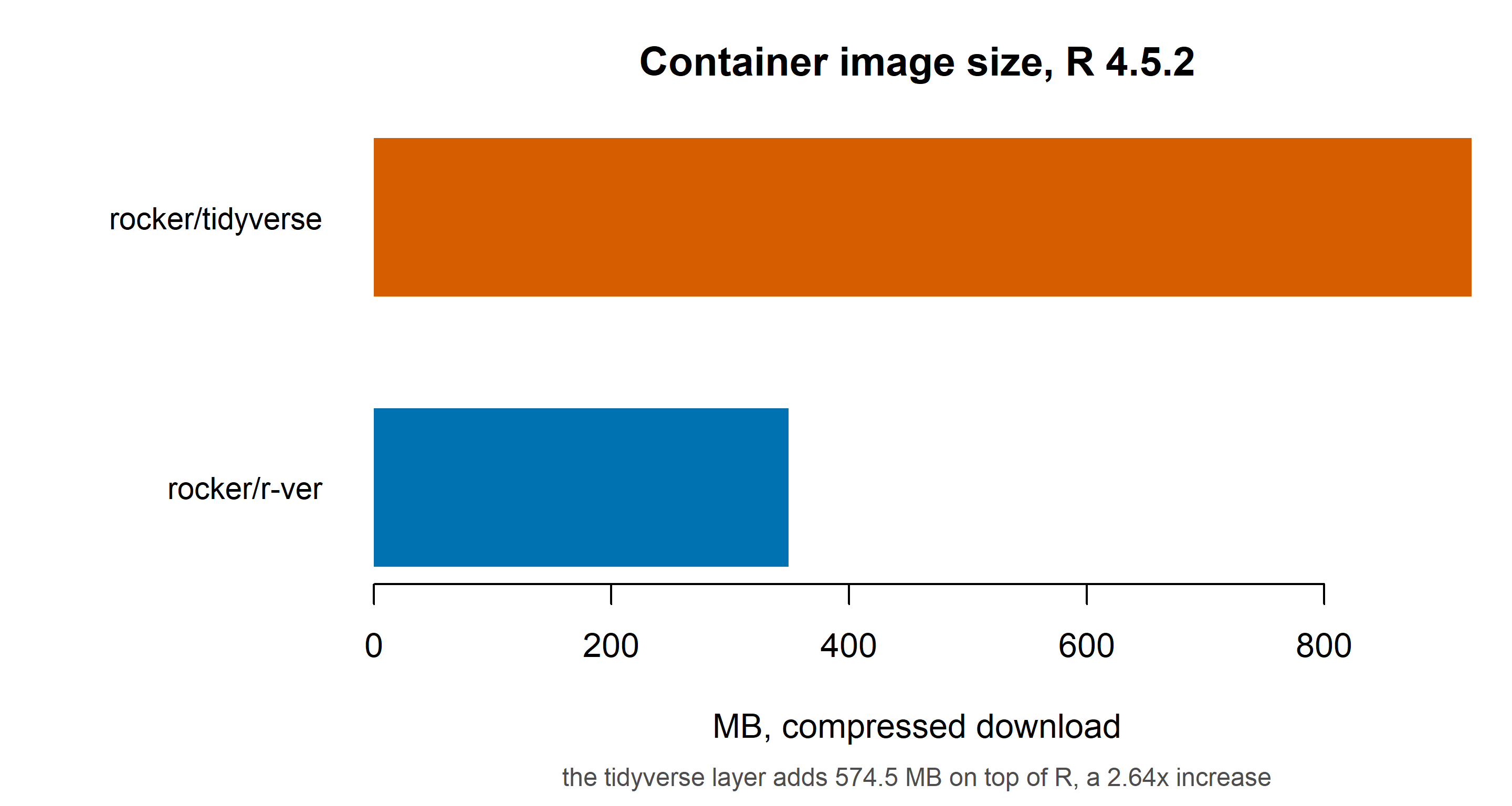
A base-R image is 349 MB; adding the tidyverse layer takes it to 924 MB. That 574 MB is not a mistake or a packaging artefact — it is the price of the dependency tree, paid on every pull, every CI run and every cold start, whether or not the code being run touches a single one of those packages.
Two caveats, both recorded in the CSV. These are Docker Hub’s reported sizes for the whole tag, which is the sum of its compressed layers — a real number a real user downloads, but not the unpacked size on disk, and the ratio is only as fair as the fact that both tags were built at the same time by the same publisher. And they are published metadata read over HTTP, not a local build: no daemon was involved, which is why this is reproducible on any machine, and also why it cannot control the comparison.
Read next to the CRAN table above, the pattern is consistent. Base graphics is not lighter by a little; it is lighter by an order of magnitude, because it inherits the empty part of R’s dependency graph rather than extending it.
1.7 What base graphics costs
An honest chapter has to state the other side.
- More typing. Base graphics is verbose by design. The same plot is longer in base than in ggplot2, and it stays that way.
- No automatic grouping or faceting. You build panels yourself with
par()orlayout()and a loop, where ggplot2 hasfacet_wrap(). Chapter 11 covers this and it is the single biggest readability jump in the book. - No automatic scale transformation. Nothing is transformed unless you name it. This is a feature when you want control and a cost when you do not.
- A smaller ecosystem. The reference grid, the grammar extensions, the themes, the colour scales: all of that ecosystem is ggplot2’s, not base’s.
- Older idiom. Base graphics code from 2001 still runs. That cuts both ways.
1.8 A decision tree
Most of the above reduces to one question: who decides what the plot looks like?
init <- par(no.readonly = TRUE)
# A flowchart is a picture, not a data plot: no axes, and the coordinates are
# laid out by hand. ps is set explicitly because text size otherwise depends on
# the device knitr happened to open, which is how a hand-placed diagram ends up
# with labels larger than its boxes.
par(xpd = NA, mar = c(0, 0, 0, 0), ps = 9)
plot.new()
plot.window(xlim = c(0, 100), ylim = c(12, 104))

box <- function(x, y, w, h, label, sub, fill) {
  rect(x, y - h / 2, x + w, y + h / 2, col = fill, border = 'grey25', lwd = 1.5)
  text(x + w / 2, y + (if (nzchar(sub)) 3.2 else 0), label, font = 2, cex = 0.92)
  if (nzchar(sub)) {
    text(x + w / 2, y - 4.6, sub, cex = 0.66, col = 'grey20')
  }
}
yes_no <- function(x, y, lab) text(x, y, lab, cex = 0.7, col = 'grey25')

Q <- '#DCE9F5'   # question
G <- '#F7E2D5'   # ggplot2 outcome
B <- '#DFF0E3'   # base outcome

box(4, 90, 52, 15, 'Is the plot final?',
    'One answer, written once, no iteration', Q)
box(4, 57, 52, 19, 'Does it have to run somewhere\nyou do not control?',
    'Locked-down server, CRAN check, minimal container', Q)
box(64, 90, 34, 15, 'ggplot2', 'Explore, iterate, facet, publish', G)
box(64, 57, 34, 15, 'ggplot2', 'Communicate, share, present', G)
box(22, 22, 52, 17, 'Base graphics',
    'Package internals, batch reports,\nexact control over the marks', B)

arrows(56, 90, 63.5, 90, length = 0.07, lwd = 1.6)
arrows(30, 82.4, 30, 66.7, length = 0.07, lwd = 1.6)
arrows(56, 57, 63.5, 57, length = 0.07, lwd = 1.6)
arrows(30, 47.4, 40, 30.7, length = 0.07, lwd = 1.6)

yes_no(59.7, 93, 'yes')
yes_no(32.4, 74.5, 'no')
yes_no(59.7, 60, 'yes')
yes_no(24, 39, 'no')

par(init)
Two questions, and note that “final” is doing more work than “simple”. A plot you will iterate on twenty times belongs to ggplot2 even if it is a single scatterplot, because the cost of base graphics is paid on every edit. A plot you will write once and run ten thousand times belongs to base graphics even if it is complicated, because that is where the per-plot cost actually lands.
Note also that the second question overrides the first. A plot that must run on a server you do not control is a base-graphics plot even if you would rather be iterating, because “install ggplot2 on this locked-down box” is not a decision you get to make.
That tree is a starting point, not a rulebook. Plenty of working code mixes the two: base graphics for the bulk of a report, one ggplot2 plot where the faceting carries the argument. The point is that the choice should be made deliberately, per plot, rather than by default.
1.9 When you have read this chapter
You now have four measured numbers and a decision tree. In the rest of the book we stop arguing and start drawing, and every chapter is written to the assumption that you want the marks exactly where you put them.
Chapter 2 surveys the three R graphics systems and walks the six dispatch cases of plot(). From Chapter 3 onward the argument is one argument at a time: here is the bare call, here is what changing pch does, here is everything combined. Nothing in this book requires installing anything.